


Who Finances Food Affordability? Agricultural Pricing and the Economic Vulnerability of Farming Households in India
Agriculture continues to occupy an important position in the Indian economy by contributing to food security, employment generation, rural livelihoods and overall socio-economic stability. A significant percentage of rural households continue to rely on agriculture despite the economy’s progressive structural transformation to becoming a services economy.
Indian farmers have done reasonably well to improve yields and expand area under cultivation. However, they are faced with natural (weather related uncertainty and consequent variation in yields and output quality) as well as market (not being able to realise even the MSP) constraints that don’t allow them to invest in their farms and families.
A typical farming family has small landholdings, poor earnings, limited asset ownership, and high indebtedness. Concurrently, the opportunity cost of staying in agriculture, caused by increasing input costs and escalating land prices, has gone up and so has the rural households’ cost of living due to rising cost of transport, healthcare and education.
Agricultural Policy: Impact on Farmers
India’s agricultural policy, like that of many nations, has historically sought to balance farm incomes, food affordability and broader development objectives. In practice, these arrangements may contribute to situations where many producers are unable to realise prices that are sufficient to cover their full economic costs.
The concern that agricultural producers bear the cost of broader development objectives has a long history in development economics. Michael Lipton[1] in his urban-bias thesis argued that development strategies frequently “squeezed” agriculture to provide cheap food and raw materials for urban constituencies. Similarly, Robert Bates documented policy regimes that diverted resources from farmers to other sectors and discriminated against agricultural producers through state interventions.[2]
We did need food to be affordable earlier and need it today too, as millions of households still need food subsidy. Affordable food, therefore, is a legitimate social objective. But so are fairness and transparency in allocation of public resources and assessment of impact of policy choices on household economics.
OECD estimates the Market Price Support (MPS) for the Indian farmers to be persistently negative since 2000, disadvantaging agriculture producers. A large negative MPS in cereals may coexist with positive support elsewhere. Some farmers may be financing food affordability, while others are protected from competition. The same policy system is simultaneously pursuing food security, inflation management, farmer support, industrial competitiveness, regional politics, and rent distribution.
The result is a second-best equilibrium, where food prices are not market prices, wages are partly adjusted to food prices, procurement prices affect planting decisions, fertiliser subsidies affect input choices, electricity subsidies affect groundwater extraction, trade restrictions affect domestic prices, food subsidies affect consumption. Every intervention creates a justification for another intervention.
A series of these interventions may contribute to farmers financing consumers, consumers financing wage competitiveness, and wage competitiveness financing business growth and profitability.
Agriculture faces weather risk, pest and disease risk, price volatility, biological production cycles, and increasing climate uncertainty. Dealing with uncertainty and managing risks requires technology, and infrastructure and the farmer must have capital to invest and tide over bad production years. Persistent extraction from the sector reduces the farmer’s ability to build capital and invest in farming and his or her family.
Over the years, many advanced economies have concluded that food production is strategic, agricultural risk is unusually high, and competitive markets alone do not always deliver stable farm incomes. They have, therefore, created direct support mechanisms like income payments, crop insurance, disaster support, decoupled payments, environmental payments, etc.
OECD’s transfer-accounting framework allows this proposition to be examined by identifying transfers among producers, consumers and taxpayers. In OECD accounting these appear as positive producer support and transfer estimates. The framework makes the transfers transparent, helps us to identify the reason for these transfers, assess their impact on efficiency and equity, etc.
We combine household economics, production uncertainty, MSP realization, and OECD[3] transfer accounting to examine whether Indian agricultural producers implicitly finance part of the country’s food-affordability objective. Rather than evaluating a particular policy instrument, the paper focuses on identifying the structure of transfers among producers, consumers, and taxpayers and assessing whether current arrangements provide adequate resources for capital formation, risk management, and household well-being within the farming community.
Agricultural Pricing: At the Core of our Problem
We study agricultural pricing from both farmer and consumer perspectives, with a focus on the Minimum Support Price (MSP) system. Our analysis identifies multiple sources of economic vulnerability, with agricultural pricing policy and its implementation being one of the important contributors. Farm Harvest Prices are often lower than MSP in many states across crops. MSP covers only a limited number of crops in any case.
The results show that while MSP has grown over time, its advantages are still concentrated in a small number of crops and geographical areas, with wheat and paddy accounting for most of the procurement. The crop-level analysis reveals substantial disparities in MSP realization and income outcomes across states, with many farmers continuing to sell below MSP and experiencing significant income losses. Even in cases where MSP is realized, the income generated is often insufficient to adequately compensate for family labour, owned land and other imputed costs.
The study concludes that fair agricultural pricing should consider farming households’ cost of living needs in addition to production costs. Agricultural pricing policy needs to be integrated with broader economic and social need for investment in human capital so that the farming families too can participate in India’s economic transformation. If not, there is a need to guarantee either affordable access to necessary services or provide higher amount of basic income support to raise an average farming family’s standard of living and help them enhance their ability to contribute to India’s economic and social progress.
1. Significance of Agriculture Sector in Indian Economy
Agriculture remains the foundation of India’s rural economy despite the country’s gradual shift towards industry and services. The sector contributes about 14% to Gross Value Added (GVA), provides food security and employs about 41% of the workforce, making it one of the largest sources of livelihood in the country (Chart 1).
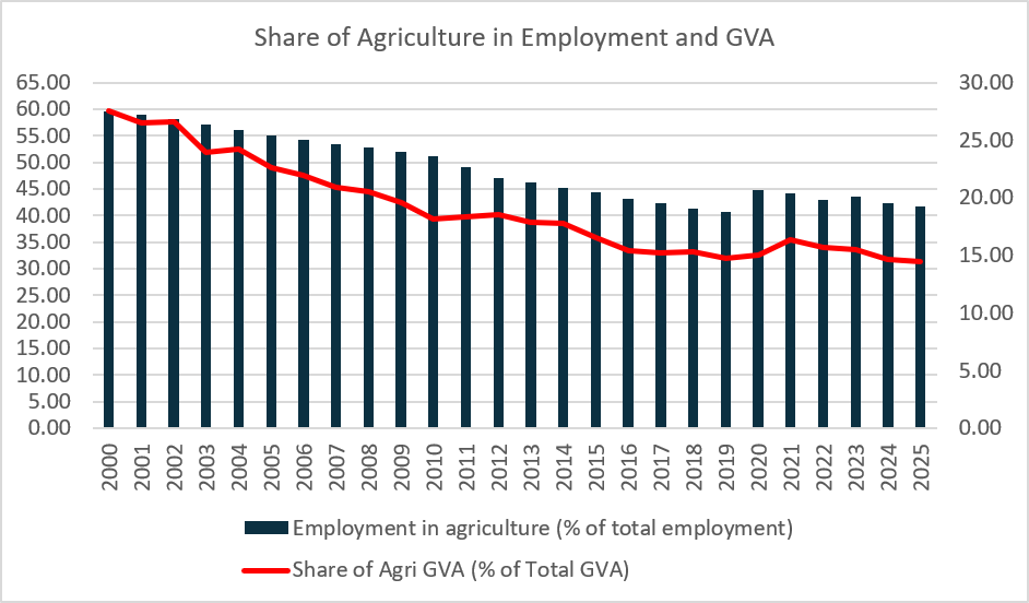 Agriculture recorded its highest growth rate of 5.51 per cent during 2010-13, followed by 4.44 per cent during 2020-23. In comparison to other sectors, growth in agriculture GVA has been relatively lower in the other periods, implying that income for households depending on agriculture has grown at rates lower than other sectors (Table 1).
Table 1: GVA Growth Rate Sector Wise in India (At Constant 2011-12 Prices)
| Year | Agriculture | Services | Manufacturing | Total Economy |
| 1991-1998 | 2.68% | 6.88% | 6.26% | 5.19% |
| 1999-2001 | 1.32% | 7.25% | 5.67% | 5.10% |
| 2002-2009 | 2.13% | 7.50% | 8.44% | 6.52% |
| 2010-2013 | 5.51% | 7.34% | 5.52% | 6.24% |
| 2014-2019 | 3.14% | 8.24% | 8.34% | 7.04% |
| 2020-2023 | 4.44% | 3.25% | 3.49% | 3.80% |
| 2024-2026 | 3.87% | 8.15% | 5.77% | 6.88% |
Source: Author’s Calculations from KLEMS database, DBIE.
It is evident from Table 2 that agriculture and allied activities recorded growth in all years from 2018-19 to 2023-24, with growth ranging from 1.40 per cent to 6.20 per cent. Notably, in 2020-21, when the economy declined by 4.10 per cent, the agriculture and allied sector grew by 4.00 per cent. However, its growth moderated in the recent years.
Table 2: Growth in value added of Agriculture and Allied Activities from 2018-19 to 2023-24
| Year | Total Economy | Agriculture & Allied Sector | Crops | Livestock | Forestry & Logging | Fishing |
| 2018 -19 | 5.80 | 2.10 | -2.40 | 8.70 | 7.60 | 8.50 |
| 2019 -20 | 3.90 | 6.20 | 5.70 | 7.50 | 6.10 | 4.50 |
| 2020 -21 | -4.10 | 4.00 | 2.60 | 6.20 | 5.80 | 3.80 |
| 2021 -22 | 9.40 | 4.60 | 3.20 | 6.40 | 0.60 | 13.00 |
| 2022 -23 | 6.70 | 4.70 | 4.70 | 5.00 | 1.00 | 8.30 |
| 2023 -24 | 7.20 | 1.40 | 2.51 | 2.90 | 1.19 | 5.21 |
Source: Ministry of Agriculture and Farmers Welfare, 2026.
Among the allied sectors, crops showed greater variation, including a negative growth of 2.40 per cent in 2018-19, which is associated with deficient monsoon rainfall and adverse weather conditions. According to the India Meteorological Department, southwest monsoon rainfall was 91 per cent of the long-period average at the all-India level, while several states experienced deficient rainfall.
Livestock and forestry recorded positive growth throughout. Fishing recorded the highest growth of 13.00 per cent in 2021-22. Overall, the data indicates differences in the growth performance of crops and allied activities across the period. During 2020-21, when the economy-wide growth was negative, agriculture contributed significantly to economic stability, with growth at 4% when the economy had experienced a negative growth.
Capital Productivity in Agriculture, though declining, continues to be higher than other sectors
Capital productivity is important because it measures how efficiently the capital invested in a sector is converted into value added. A higher capital productivity indicates greater value added generated per unit of capital (Annual GVA/Capital Stock), making it a useful indicator for comparing the efficiency of capital utilisation across sectors and over time (Table 3).
Table 3: Capital Productivity Sector-wise in India (period wise average)
| Period | Agriculture | Services | Manufacturing | Economy |
| 1991-1998 | 0.58 (3.47, 2.33) | 0.26 (7.11, 4.67) | 0.33 (7.44, 8.92) | 0.34 (5.76, 4.93) |
| 1999-2001 | 0.60 (2.96, 4.52) | 0.29 (5.73, 8.07) | 0.28 (4.57, 4.52) | 0.27 (4.51, 6.38) |
| 2002-2009 | 0.54 (3.00, 4.58) | 0.28 (7.82,8.13) | 0.28 (9.09, 8.91) | 0.33 (7.05, 7.93) |
| 2010-2013 | 0.48 (4.46, 5.23) | 0.27 (7.28, 8.31) | 0.28 (4.59, 5.59) | 0.31 (5.58, 7.67) |
| 2014-2019 | 0.46 (4.43, 3.51) | 0.27 (7.56, 7.61) | 0.30 (6.06, 5.15) | 0.30 (6.39, 6.70) |
| 2020-2023 | 0.47 (3.09, 3.48) | 0.25 (6.30, 4.36) | 0.30 (2.45, 3.31) | 0.28 (5.28, 4.06) |
Source: Author’s Calculations from KLEMS Database, Note: Figures in parenthesis are: CAGR of GVA, and CAGR of capital Stock, respectively.
Agriculture recorded higher capital productivity than services, manufacturing and the overall economy in every period, indicating that it generated comparatively higher value added per unit of capital. Its capital productivity increased from 0.58 in 1991-1998 to a peak of 0.60 during 1999-2001 but subsequently declined to 0.47 during 2020-2023.
The decline suggests that capital accumulation was not accompanied by a proportionate increase in GVA in several periods, particularly during 2002-2009, when capital stock grew by 4.58 per cent compared with GVA growth of 3.00 per cent – period that coincides with some of the lowest increases in MSP for food as well as non-food crops. Despite this decline, agriculture continued to maintain higher capital productivity than the other major sectors.
When it comes to employment growth sector-wise (Table 4), agriculture recorded low or negative employment growth in most periods, particularly during 2002-2009, 2010-2013 and 2014-2019, implying increased labour productivity The increase in employee growth rate during 2020-2023 is due to reverse migration of the people during COVID-19.
Table 4: Growth rate of Employment Sector-wise
| Year | Agriculture | Construction | Trade | Transport & Storage | Financial Services | Business Services | Education | Health & Social Work |
| 1991-1998 | 1.02% | 3.07% | 3.86% | 4.16% | 3.35% | 9.34% | 4.50% | 3.81% |
| 1999-2001 | 0.57% | 5.87% | 3.90% | 4.80% | 2.65% | 11.28% | 4.99% | 5.39% |
| 2002-2009 | -0.42% | 8.96% | 2.43% | 3.41% | 6.19% | 10.19% | 4.73% | 4.47% |
| 2010-2013 | -1.95% | 7.90% | 1.40% | 2.69% | 4.93% | 9.56% | 3.39% | 3.81% |
| 2014-2019 | -1.32% | 2.67% | 2.68% | 3.25% | 4.80% | 8.76% | 4.72% | 5.74% |
| 2020-2023 | 3.25% | 6.29% | 1.46% | 0.04% | 1.81% | 8.25% | -1.23% | 7.73% |
Source: Author’s Calculations from KLEMS Database
However, the sector continued to record positive GVA growth, while its capital productivity remained higher than that of the other sectors throughout the periods considered. Thus, agriculture generated value with comparatively higher capital productivity and improving labour productivity (Table 5 below).
Table 5: GVA/Employed Person in INR Lakhs by Sector (Period Average)
| Period | Agriculture | Services | Manufacturing | Total Economy |
| 1991-1998 | 3.78 (1.64%) | 14.50 (3.02%) | 11.25 (4.48%) | 7.76 (3.38%) |
| 1999-2001 | 4.38 (0.75%) | 17.70 (3.48%) | 13.68 (2.93%) | 13.68 (3.29%) |
| 2002-2009 | 4.80 (2.56%) | 21.97 (4.32%) | 17.40 (6.24%) | 12.24 (5.11%) |
| 2010-2013 | 6.30 (7.62%) | 28.51 (4.63%) | 25.16 (4.70%) | 16.79 (5.59%) |
| 2014-2019 | 8.28 (4.52%) | 36.85 (4.52%) | 35.73 (8.22%) | 22.86 (6.10%) |
| 2020-2023 | 8.69 (1.74%) | 38.38 (-0.20%) | 40.70 (-0.84%) | 24.01 (0.09%) |
| Overall CAGR | 2.87% | 3.51% | 4.49% | 4.01% |
Source: Author’s Calculations from KLEMS Database, figures in parenthesis are CAGR of GVA/Employed person.
Agriculture shows a continuous improvement in GVA per employed person, increasing from 3.78 lakhs during 1991-1998 to 8.69 during 2020-2023. Its overall CAGR was 2.87 per cent, which was lower than services (3.51%), manufacturing (4.49%) and the total economy (4.01%), indicating slower long-term growth in agricultural labour productivity. The highest CAGR in agriculture was recorded during 2010-2013 at 7.62 per cent (a period that coincided with large increases in MSP for food as well as non-food crops), but it moderated substantially to 1.74 per cent during 2020-2023. Thus, agricultural labour productivity increased in absolute terms, but its pace of growth slowed in the recent period, largely on account of increased household dependence on agriculture for employment as mentioned earlier. In contrast, manufacturing recorded the highest GVA per employed person at 40.70 during 2020-2023, although its recent CAGR was negative at -0.84 per cent.
The broader context of agricultural growth is better understood by examining the structural transformation of the Indian economy. It is evident from Table 6, During 2000-01 to 2022-23, agriculture recorded an annual Gross Value Added (GVA) growth of 3.50%, considerably lower than sectors such as construction (7.26%), trade (7.43%), education (8.49%) and health and social work (8.46%). While agricultural labour productivity increased by 3.31% annually, indicating improvements in production efficiency, the relatively slower growth of agriculture compared with other sectors highlights the changing structure of the Indian economy. Despite this transformation, agriculture continues to support a disproportionately large share of the workforce, suggesting that improvements in agricultural production and productivity have not been accompanied by a comparable improvement in the sector’s relative economic position.
Table 6: Structural Transformation Indicators Across Major Sectors in India (2000-01 to 2022-23)
| Sector | GVA CAGR | Labour Quality CAGR | Labour Productivity CAGR | Labour Income Share (VA) Change | Labour Income Share (GO) Change |
| Agriculture | 3.50 | 0.32 | 3.31 | 0.00 | 0.03 |
| Construction | 7.26 | 0.29 | 0.67 | -0.03 | -0.02 |
| Trade | 7.43 | 0.47 | 4.51 | -0.02 | -0.05 |
| Financial Services | 6.82 | 0.38 | 1.90 | -0.05 | -0.05 |
| Education | 8.49 | 0.27 | 4.77 | -0.02 | -0.05 |
| Health & Social Work | 8.46 | 0.46 | 3.36 | 0.06 | 0.06 |
Source: India KLEMS Database, 2026
2. Growth and Variability in Agricultural Production
In this section we examine the growth, productivity and variability of food grains and non-food grains production. We also examine the relationship between rainfall deviations and crop production, highlighting the risk and uncertainty in agriculture.
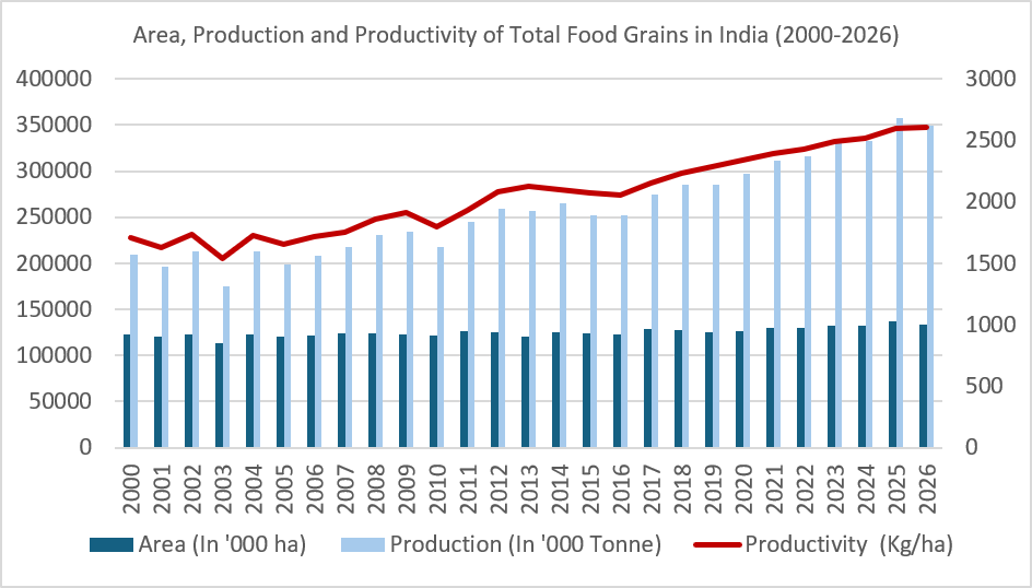
The record foodgrain production of 357.73 million metric tonnes during 2023-24 and the sustained expansion of horticultural production to 362.08 million tonnes (Press Information Bureau, 2026), demonstrates the sector’s growing production capacity and diversification. Over the past two decades, the agriculture sector has recorded steady growth in production of food grains (2.05 per cent) and productivity (1.72 per cent), whereas the cultivated area has remained nearly constant, growing by only 0.33 per cent (Chart 2).
Chart 2: Area, Production and Productivity of Total Food Grains in India
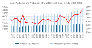
In case of non-food grains, production, productivity grew at 1.33 per cent, 0.29 per cent and area at 1.03 per cent, respectively (Chart 3).
Chart 3: Area, Production and Productivity of Total Non-Food Grains in India
An analysis of performance across eras (table 7) suggests that increases in food-grain production have been achieved predominantly through productivity improvement and not through substantial expansion of cultivated area.
Table 7: CAGR of Area, Production and Yield of Food Grains and Non-Food Grains in India
| Year | Area | Production | Yield | |||
| FG | NFG | FG | NFG | FG | NFG | |
| 1991-1998 | -1.75% | 0.85% | 0.75% | 3.54% | 2.54% | 2.67% |
| 1999-2001 | -1.66% | -4.89% | -1.68% | -1.73% | -0.03% | 3.32% |
| 2002-2009 | 0.01% | 1.58% | 1.39% | 0.70% | 1.38% | -0.87% |
| 2010-2013 | -0.15% | 2.44% | 5.64% | 3.51% | 5.79% | 1.04% |
| 2014-2019 | -0.04% | -1.12% | 1.48% | -0.38% | 1.70% | 0.75% |
| 2020-2022 | 1.24% | 3.93% | 3.00% | 8.58% | 1.73% | 4.47% |
| 2023-2026 | 0.37% | -1.48% | 1.88% | 1.44% | 1.50% | 2.96% |
| Overall | -0.14% | 0.88% | 1.87% | 1.86% | 2.01% | 0.97% |
Source: Author’s calculations from Ministry of Agriculture and Farmers Welfare.
Overall, food-grain area declined marginally at a CAGR of 0.14%, while production and productivity increased by 1.87% and 2.01%, respectively. The strongest improvement was recorded during 2010-2013, when production and productivity grew by 5.64% and 5.79%, respectively, despite a marginal decline in area. The recent period also reflects continued productivity-led growth, with food-grain production increasing by 1.88% during 2023-2026 with area growth of only 0.37%.
At this stage, the gains in productivity and production may become increasingly difficult to sustain without continued technological advancement, improved crop varieties, irrigation and other productivity-enhancing investments., which require substantial investment. However, such investments remain difficult to make for most farmers, as a large proportion of them are economically poor.
Table 8: Variability (Coefficient of Variation or CV) in Yield of Food Grains, Non-Food Grains
| Years | Food Grains | Non-Food Grains |
| 1991-1998 | 6.66% | 4.44% |
| 1999-2001 | 2.71% | 3.32% |
| 2002-2009 | 6.66% | 3.28% |
| 2010-2013 | 7.55% | 1.41% |
| 2014-2019 | 4.66% | 2.85% |
| 2020-2022 | 1.73% | 4.41% |
| 2023-2026 | 2.29% | 3.16% |
Source: Authors calculations from Ministry of Agriculture and Farmers Welfare.
The variability estimates (Table 8) above demonstrated that agricultural production operates under a risk-prone production environment, reflected in fluctuations in both rainfall and crop productivity across periods. Food-grain productivity recorded a CV as high as 7.55 per cent during 2010-2013. Non-food-grain productivity also exhibited substantial variation in several periods, with its CV reaching 4.41 per cent during 2020-2022. The variability is not uniform across periods, indicating that farmers face changing production conditions rather than a stable production environment. Such fluctuations are particularly important for farm households because production outcomes are determined before farmers know the conditions under which their output will be realised.
In order to know the effect of rainfall on production, we have considered years with rainfall deviation exceeding 10 per cent to examine the corresponding decline in food grain production (table 9). The results show that the selected rainfall-deficit years were followed by declines in total food grain production, with the decline being highest at 17.89 per cent in 2002-03, followed by 6.95 per cent in 2004-05, 6.98 per cent in 2009-10, 4.91 per cent in 2014-15 and 0.18 per cent in 2015-16. The crop-wise results also show considerable variation, with the magnitude of production change differing across rice, wheat, coarse cereals and pulses. The relatively large decline in 2002-03 is particularly notable, as years preceding had also received less rainfall. These rainfall deviations are associated with substantial variation in subsequent food grain production, although the magnitude of the response differs across crops and years.
Table 9: Rainfall Deviation and Subsequent Decline in Food Grain Production in India
| Year | Production decline in Following Year (%) | |||||
| Rain Deviation | TFG | Rice | Wheat | Coarse cereals | Pulses | |
| 2002 | -19.20 | 17.89% | 23.08% | 9.63% | 21.88% | 16.75% |
| 2004 | -13.80 | 6.95% | 6.10% | -1.03% | 11.01% | 11.94% |
| 2009 | -21.80 | 6.98% | 10.17% | -0.15% | 16.21% | -0.62% |
| 2014 | -11.90 | 4.91% | 1.10% | 9.72% | 0.99% | 10.91% |
| 2015 | -14.00 | 0.18% | 1.01% | -6.66% | 10.13% | 4.84% |
Source: Author’s calculations from various government reports.
The coexistence of rising production, improving productivity and continued vulnerability of farming households suggests that aggregate agricultural growth alone may not be sufficient to improve household economic resilience. Consequently, the prices and the cost of cultivation become the most important determinants of farmer income and surplus.
3. Rationale for Examining Fairness in Agricultural Pricing
Farming involves committing land, labour and other resources under uncertain climatic and production conditions, while the returns are realised only after the production process is completed. Climate conditions establish both the production environment and agricultural outcomes that exhibit measurable variability. This uncertainty distinguishes agriculture from many other economic activities.
Rising production costs, climate uncertainty, volatile markets and fragmented landholdings further weaken farm incomes. Agriculture is inherently seasonal, resulting in fluctuations in labour requirement throughout the year. Consequently, a large proportion of the rural workforce remains engaged in agriculture even when labour requirements are low, leading to disguised employment, lower labour productivity and relatively low farm incomes. Limited non-farm part-time employment opportunities further constrain the ability of farming households to diversify their sources of income.
As agricultural production, productivity and cultivated area increase, the economic benefits accruing to farmers depend on whether the prices received for their produce increase in line with costs. Since agricultural markets are characterized by seasonal fluctuations, varying demand and supply conditions, and differences in market access, the prices realized by farmers may differ substantially across crops, regions and marketing channels. Consequently, agricultural pricing policies, including the Minimum Support Price (MSP), have an important role in influencing farmers’ income, price stability and consumer welfare.
Although previous studies have examined agricultural pricing, MSP, procurement systems and cultivation costs from different perspectives, relatively limited attention has been given to whether the existing pricing framework enables farming households to earn adequate income to meet essential household needs such as education, healthcare, housing and other basic living expenses while balancing consumer interests.
In light of this, the present study attempts to examine the concept of fairness in agricultural pricing from both producer and consumer viewpoints by analysing the extent to which farmers benefit from the existing price support framework, evaluating consumer concerns regarding food prices, and comparing the socio-economic conditions of rural and urban households using secondary data from official government sources.
4. Variability in FHP, MSP and Farm Earnings
We have examined the variability in Farm Harvest Prices (FHP), Minimum Support Prices (MSP), and farm earnings across selected crops and states to compare the variability in prices received by farmers with changes in MSP. We further estimated farm earnings after C2 costs to assess how price variations affect farm returns. This provides a basis for understanding the stability and adequacy of farm earnings across crops and states.
4.1 Variability in Farm Harvest Price
In a world where MSP system is working as intended, the difference between FHP and MSP should be near zero. Since farm earnings depend directly on the price received for the produce, such fluctuations can contribute to instability in farm returns. When considered along with the observed variability in farm earnings, the findings suggest that price instability is possibly one of the factors associated with the declining attractiveness of farming as a livelihood. The results in table 10 shows considerable variation in Farm Harvest Prices (FHP) across the selected crops and states during 2017-18 to 2022-23. The coefficient of variation was particularly high for paddy in Punjab (23.84%), bajra in Maharashtra (23.25%) and Mustard in Bihar (23.15%), while lower variability was observed for wheat in Himachal Pradesh (4.61%) and gram in Gujarat (5.90%). The differences in Min-Max values further indicate that the extent of price fluctuation varied considerably across crops and states. Since FHP represents the prices realised by farmers, greater FHP variability implies greater uncertainty in household incomes, which influences farmers’ production and marketing decisions.
Table 10: FHP and MSP Variability 2017-18 to 2022-23:
| Best Productive states | ||||||
| Crop | State | FHP Min-Max (INR/quintal) | FHP CV (%) | State | FHP Min-Max (INR/quintal) | FHP CV (%) |
| Paddy | Punjab | 1,596-2,924 | 23.84 | AP | 1,559-1,997 | 8.41 |
| Wheat | Punjab | 1,640-2,025 | 7.34 | Haryana | 1,735-2,173 | 8.11 |
| Maize | AP | 1,204-1,957 | 15.91 | Telangana | 1,323-1,815 | 11.07 |
| Bajra | Gujarat | 1,195-2,090 | 17.9 | Maharashtra | 1,282-2,383 | 23.25 |
| Gram | AP | 4,060-4,810 | 6.49 | Gujarat | 3,842-4,457 | 5.9 |
| Groundnut | Rajasthan | 3,716-6,011 | 17.52 | Telangana | 3,941-6,196 | 17.19 |
| Mustard | MP | 3,840-5,872 | 17.76 | Gujarat | 3,518-5,463 | 20.22 |
| Least Productive states | ||||||
| Paddy | Jharkhand | 1,279-1,635 | 7.88 | Maharashtra | 1,741-2,250 | 8.96 |
| Wheat | HP | 2,085-2,387 | 4.61 | Jharkhand | 1,742-2,159 | 8.32 |
| Maize | Gujarat | 1,376-2,056 | 13.62 | HP | 1,887-2,247 | 6.16 |
| Bajra | Rajasthan | 1,258-1,994 | 16.5 | UP | 1,152-1,926 | 17.21 |
| Gram | Karnataka | 3,758-4,798 | 9.04 | Chhattisgarh | 4,446-6,239 | 12.17 |
| Groundnut | Odisha | 3,883-6,127 | 17.48 | Karnataka | 3,638-6,379 | 21.11 |
| Mustard | Assam | 2,898-3,414 | 6.98 | Bihar | 3,221-5,653 | 23.15 |
Source: Author’s calculations from Ministry of Agriculture and Farmers Welfare
4.2 Variability in Farm Earnings
We have estimated farm earnings after C2 at FHP for selected crops and states for the period 2017-18 to 2022-23 to examine both the level and variability of farm returns in table 11, the results show that higher productivity does not necessarily translate into higher or stable farm earnings.
Several selected high-productivity states recorded considerable variability in earnings, such as maize and gram in Andhra Pradesh, with coefficient of variation (CV) of 80.97 per cent and 157.64 per cent, respectively. Even states with relatively high average earnings showed substantial variability, as observed for paddy in Punjab and groundnut in Rajasthan, with variation of 58.29 per cent and 53.36 per cent, respectively.
We also observe negative average earnings after C2 for several crop-state combinations, including paddy in Jharkhand, maize in Gujarat and groundnut in Odisha, indicating that the price realised at FHP did not cover C2 costs on average during the period.
Further, earnings from the same crop differed considerably across states, highlighting differences in farm returns. Exceptionally high CVs, such as 1,419 per cent for bajra in Rajasthan and 427.70 per cent for maize in Telangana, are associated with very low average earnings, making relative variability particularly high.
Overall, our estimates show that farm returns depend not only on productivity but also on the relationship between the price received by farmers and the comprehensive cost of cultivation. With considerable change in both the level and risk of farm earnings across crops and states, it is not easy for farmers to build the capital required for investment.
Table 11: Variability in farm earnings after C2 at FHP, from 2017-18 to 2022-23
| Crop | State | Average | Std Dev | Coeff of Variation | State | Average | Std Dev | Coeff of Variation |
| Best Productive states | ||||||||
| Paddy | Punjab | 47,316 | 27,579 | 58.29% | AP | 13,418 | 4,941 | 36.82% |
| Wheat | Punjab | 20,612 | 7,265 | 35.25% | Haryana | 29,543 | 7,372 | 24.95% |
| Maize | AP | 25,456 | 20,613 | 80.97% | Telangana | 1,128 | 4,823 | 427.70% |
| Bajra | Gujarat | 6,815 | 7,392 | 108.47% | Maharashtra | -10,648 | 5,412 | -50.83% |
| Gram | AP | 7,146 | 11,264 | 157.64% | Gujarat | 5,568 | 9,647 | 173.25% |
| Groundnut | Rajasthan | 38,123 | 20,342 | 53.36% | Telangana | -24,334 | 7,014 | -28.82% |
| Mustard | MP | 29,165 | 9,679 | 33.19% | Gujarat | 14,853 | 12,378 | 83.34% |
| Least productive states | ||||||||
| Paddy | Jharkhand | -5,274 | 5,405 | -102% | Maharashtra | -30,887 | 3,139 | -10% |
| Wheat | HP | -6,168 | 7,987 | -129% | Jharkhand | -13,801 | 7,458 | -54% |
| Maize | Gujarat | -8,250 | 4,173 | -51% | HP | 5,962 | 3,542 | 59% |
| Bajra | Rajasthan | 172 | 2,441 | 1419% | UP | 687 | 687 | 100% |
| Gram | Karnataka | 7,146 | 11,264 | 158% | Chhattisgarh | 5,568 | 9,647 | 173% |
| Groundnut | Odisha | -22,662 | 3,202 | -14% | Karnataka | -5,685 | 9,172 | -161% |
| Mustard | Assam | -7,077 | 2,036 | -29% | Bihar | 4,696 | 2,041 | 43% |
Source: Author’s calculation from CACP reports.
The findings, therefore, highlight that farm earnings are subject to fluctuations arising from variations in both production and pricing conditions, which indicates that irrespective of the agriculture sector’s relevance and significant, it is prone to large variations in earnings making rural households vulnerable to uncertainty in production as well as the market environment.
5. How far has growth in agriculture output and value-addition improved farmers’ lives?
This section examines the socio-economic characteristics of farming households, including landholding size, livelihood diversification, income composition, financial vulnerability, market security and essential household expenditure, to provide a comprehensive assessment of farmers’ economic conditions.
5.1 Small Holdings limit a family’s Capacity to absorb Production and Market Risk
Land is the primary productive asset in agriculture and largely determines a household’s capacity to generate income, which, in turn, determines its ability to invest in improved technologies and withstand production and market uncertainties. The extent to which farming households can benefit from agricultural growth depends not only on yield and prices but also on the size of their operational holdings, as smaller farms often have limited marketable surplus and lower capacity to absorb adverse shocks.
Understanding the distribution of land among agricultural households, therefore, provides the basis for examining the structural constraints affecting farmers’ livelihoods.
Table 12: Estimated Number of Rural Households in India
| Category | Estimated Number (Million) | Percentage of Rural Households |
| Agricultural households | 93 | 54 |
| Non-agricultural households | 79 | 46 |
| Total rural households | 172 | 100 |
Source: NSS Report No. 587, 2019.
Table 12 indicates that agriculture continues to the principal source of livelihood for more than half of the rural population, highlighting its continued socio-economic importance.
The dependence of rural households on agriculture is further compounded by a highly fragmented landholding structure (Table 13). Among agricultural households, 70.4 per cent possess less than one hectare of land, while only 0.4 per cent own more than ten hectares. Small land holdings constrain the scale of production, restrict marketable surplus, and reduce the farmers’ capacity to invest in improved technologies or withstand production and market shocks.
Table 13: Land Possessed by Rural Households in India
| Land Possession Category | Agricultural Households (%) | Non-agricultural Households (%) | Rural Households (%) |
| Less than 1 ha | 70.40 | 98.90 | 83.50 |
| More than 10 ha | 0.40 | 0.00 | 0.20 |
Source: NSS Report No. 587, 2019.
On average, an agricultural household owned only 0.88 ha of land during 2018-19, while 70.4 per cent belonged to the marginal landholding category and only 0.2 per cent owned large holdings as in table 14, Such a fragmented landholding structure limits the scale of cultivation and the potential to generate adequate farm income. Consequently, the average monthly net receipt from crop production was only INR 3,058, contributing about 36.7 per cent of the total monthly household income of INR 8,337 (Table 15).
Table 14: Household Ownership Holdings of Land During 2018-19
| Indicator | Rural Households | Agricultural Households | Non-agricultural Households |
| Average area owned per household (ha) | 0.51 | 0.88 | 0.09 |
| Landless households (%) | 8.20 | 2.60 | 14.80 |
| Marginal ownership category (%) | 76.50 | 70.40 | 83.70 |
| Large ownership category (%) | 0.10 | 0.20 | 0.00 |
Source: NSS Report No. 587, 2019.
In comparison, wage income (INR 4,063) constituted the largest source of household earnings, accounting for nearly 48.7 per cent of total income, while income from livestock (INR 441), non-farm business (INR 641) and leasing out land (INR 134) contributed relatively smaller shares.
Table 15: Average Monthly Income from Different Sources per Agricultural Household
| Source of Income | Amount (INR) | Share in total monthly income (%) |
| Income from wages | 4,063 | 48.73 |
| Income from leasing out land | 134 | 1.61 |
| Net receipt from crop production | 3,058 | 36.68 |
| Net receipt from farming of animals | 441 | 5.29 |
| Net receipt from non-farm business | 641 | 7.69 |
| Total monthly income | 8,337 | 100 |
Source: NSS Report No. 587, 2019.
These findings suggest that crop cultivation alone is insufficient to sustain the livelihoods of many agricultural households, leading them to depend on wage employment and other supplementary income sources. The coexistence of small landholdings and limited crop income highlights the economic vulnerability of farming households and underscores the importance of an agricultural pricing system that enables cultivation to provide sustainable and remunerative livelihoods.
5.2. Diversified Livelihoods, given the Limited Farm Income
Although agriculture remains the principal occupation for a majority of rural households, household income is generated from multiple economic activities.
The livelihood profile of agricultural households extends beyond crop cultivation. As shown in Table 16, while crop production remains the predominant household classification (68.9%), a sizeable proportion of agricultural households are engaged in casual labour (14.2%), regular wage employment (7.7%), non-agricultural enterprises (4.8%) and livestock farming (2.3%).
Table 16: Distribution of Agricultural Households by Household Classification and Size of Land
| Household Classification | Agricultural Households (%) | Non-agricultural Households (%) | Rural Households (%) |
| Crop production | 68.90 | 6.10 | 40.00 |
| Livestock farming | 2.30 | 0.60 | 1.50 |
| Other agricultural activities | 0.60 | 1.10 | 0.80 |
| Non-agricultural enterprise | 4.80 | 14.00 | 9.00 |
| Regular wage employment (agriculture) | 1.20 | 2.70 | 1.90 |
| Regular wage employment (non-agriculture) | 6.50 | 15.00 | 10.40 |
| Casual labour (agriculture) | 5.90 | 23.80 | 14.10 |
| Casual labour (non-agriculture) | 8.30 | 24.80 | 15.90 |
| Others | 1.60 | 11.90 | 6.30 |
Source: NSS Report No. 587, 2019.
The presence of multiple livelihood activities suggests that cultivation alone is often insufficient to meet household income requirements, leading many farming households to supplement their earnings through wage employment and other non-farm activities. This livelihood pattern highlights the economic constraints faced by agricultural households and underscores the importance of examining whether returns from cultivation are adequate to sustain rural livelihoods.
Assessing the adequacy of farm income requires examining the relationship between cultivation expenditure and the receipts generated from agricultural activities, Table 17 presents the average monthly paid-out expenditure and corresponding receipts from crop production and livestock farming among agricultural households. On average, receipts from crop production amounted to INR 6,960 against a paid-out expenditure of INR 2,959, while livestock farming generated receipts of INR 3,704 with a paid-out expenditure of INR 1,267. Although receipts exceeded paid-out expenses for both activities, these estimates reflect returns over cash expenditures only. They do not account for imputed costs, including the value of family labour, rental value of owned land and interest on fixed capital, which constitute a substantial share of the total cost of cultivation.
Table 17: Average Monthly Paid-out Expenditure and Receipts for Crop Production and Farming of Animals
| Particulars | Amount (INR) |
| Paid-out expenditure for crop production | 2,959 |
| Receipts from crop production | 6,960 |
| Paid-out expenditure for farming of animals | 1,267 |
| Receipts from farming of animals | 3,704 |
Source: NSS Report No. 587, 2019.
The economic sustainability of farming cannot be assessed solely on the basis of occupation or returns over paid-out expenditure. A comprehensive evaluation requires examining whether the income generated from cultivation is sufficient to cover the full cost of production and support household livelihoods. The dependence on wage employment and other non-farm activities indicates that cultivation alone does not provide adequate income, even where agricultural production has increased.
5.3 Financial Vulnerability of Agricultural Households
The economic well-being of agricultural households is influenced not only by the income generated from cultivation but also by their financial capacity to manage production risks and market uncertainties. Dependence on credit, access to remunerative markets and availability of risk protection mechanisms determine whether farming households can sustain agricultural operations during adverse conditions. These institutional factors, therefore, provide an important context for assessing the adequacy of agricultural prices and farmers’ economic resilience.
Table 18 below suggests that nearly half (50.2%) of all agricultural households were indebted, with an average outstanding loan of INR 74,121 per household, indicating that borrowing forms an important component of household financial management. Institutional agencies accounted for 69.6 per cent of total borrowings, suggesting that formal credit institutions play a significant role in meeting farmers’ credit requirements.
Table 18: Indebtedness of Agricultural Households
| Indicator | Value |
| Percentage of indebted agricultural households | 50.20 |
| Average outstanding loan amount per agricultural household (INR) | 74,121 |
| Institutional share in loans (%) | 69.60 |
| Loans taken for agricultural purposes (%) | 57.50 |
| Loans from agricultural professional moneylenders (%) | 20.50 |
Source: NSS Report No. 587, 2019.
At the same time, 57.5 per cent of loans were obtained for agricultural purposes, reflecting the continued dependence of farming households on external finance to meet cultivation-related expenses. Despite the predominance of institutional lending, 20.5 per cent of agricultural loans were still sourced from professional moneylenders, indicating that a section of farmers continues to rely on informal credit channels.
The broader financial position of agricultural households can be understood by examining their asset ownership and access to institutional credit. As shown in Table 19, although almost all rural and agricultural households owned some form of asset (99.4%), the average value of their total assets (INR 15.92 lakh) was substantially lower than that of urban self-employed households (INR 27.17 lakh). The disparity was particularly pronounced in financial assets, indicating relatively weaker financial resilience among agricultural households. In addition, the incidence of indebtedness was higher (40.3%), and the share of institutional credit was lower (66.1%) than among urban self-employed households. These findings suggest that despite owning productive assets, agricultural households have comparatively limited financial resources to absorb income and production shocks.
Table 19: Economic Status, Indebtedness and Credit Access of Households in India
| Indicator | Rural Households | Urban Households |
| Households owning any asset (%) | 99.40 | 98.00 |
| Households owning physical assets (%) | 97.50 | 85.40 |
| Households owning financial assets (%) | 96.60 | 94.70 |
| Average value of total assets per household (INR Lakhs) | 15.92 | 27.17 |
| Average value of physical assets per household (INR Lakhs) | 15.20 | 24.65 |
| Average value of financial assets per household (INR Lakhs) | 0.73 | 2.52 |
| Incidence of indebtedness (%) | 40.30 | 27.50 |
| Debt-Asset Ratio (%) | 3.80 | 4.40 |
| Institutional credit in outstanding cash debt (%) | 66.10 | 87.10 |
Source: compiled from NSS Report No. 588, 2019.
5.4 Farmers’ Participation in Formal Procurement System
As discussed in Section 4.3, the farm harvest prices (FHP) are often below the minimum support price (MSP). One of the possible reasons for FHP being lower than MSP is that a large proportion of farmers remain outside formal procurement systems. As shown in Table 20, over 70% of paddy, arhar, cotton and groundnut are sold through local markets, whereas only a small proportion is sold to government procurement agencies. Consequently, many farmers are more likely to receive prevailing market prices than the Minimum Support Price (MSP), limiting the effectiveness of the MSP system in ensuring remunerative prices. The concentration of crop sales in local markets, therefore, suggests that market access, rather than the announcement of MSP alone, largely determines the prices realized by farmers.
Table 20: Major Agency of Disposal of Crops by Agricultural Households (July-December 2018)
| Crop | Local Market (%) | APMC Market (%) | Government Agency (%) | Private Processors (%) |
| Paddy | 75.10 | 3.20 | 7.30 | 3.60 |
| Arhar (Tur) | 76.00 | 12.40 | 1.20 | 4.30 |
| Cotton | 71.80 | 8.90 | 2.40 | 8.80 |
| Groundnut | 73.50 | 11.90 | 1.10 | 6.90 |
| Sugarcane | 15.60 | 2.20 | 10.10 | 37.60 |
Source: NSS Report No. 587, 2019.
The vulnerability of agricultural households is further compounded by limited adoption of crop insurance. Across major crops, lack of awareness about crop insurance and its availability emerged as the most frequently reported reasons for non-participation (table 21). Combined with high indebtedness and limited access to government procurement, inadequate risk protection increases farmers’ exposure to production and price shocks. Taken together, these findings indicate that the economic fragility of farming households is driven not only by low and uncertain farm incomes but also by limited institutional support.
Table 21: Reasons for Not Insuring Crops by Agricultural Households
| Reason | Paddy (%) | Maize (%) | Soyabean (%) | Cotton (%) |
| Not aware about crop insurance | 44.20 | 47.60 | 44.20 | 34.40 |
| Not aware about availability | 15.60 | 15.80 | 11.10 | 11.90 |
| Not interested | 21.10 | 17.90 | 17.40 | 26.30 |
| No need felt | 3.40 | 3.60 | 3.50 | 3.80 |
| Insurance facility not available | 3.80 | 4.20 | 2.10 | 2.20 |
Source: NSS Report No. 587, 2019.
Our analysis so far suggests that growth in agricultural output and value addition has not been accompanied by a uniform improvement in the economic conditions of farming households. Small and fragmented holdings, limited contribution of crop income to total household income, indebtedness, dependence on supplementary livelihoods, limited access to formal markets and inadequate crop-insurance awareness remain evident in the data.
These characteristics suggest that economic vulnerability arises not from a single factor but from the interaction of limited land resources, low farm income, dependence on supplementary livelihoods and constrained ability to accumulate capital.
6. Who Finances Food Affordability? Evidence from OECD Agricultural Support Estimates
The current section examines the extent to which agricultural policy transfers have supported Indian farmers and consumers, using the OECD Agricultural Policy Monitoring and Evaluation framework, which estimates producer (PSE), general services (GSSE) and consumer (CSE) gross transfers or support to agriculture from consumers and taxpayers arising from government policies that support agriculture. We use OECD estimates as evidence for a broader argument about transparency, incidence (who bears the cost), capital accumulation, risk sharing, and fairness in burden allocation.
Producer Support (PSE)[1], measured at farm gate level, comprise market price support (MPS), budgetary payments and the cost of revenue foregone. A positive PSE indicates net support to producers, while negative PSE indicates an implicit tax or net transfer away from producers through agricultural policies.
MPS is positive when the domestic price is higher than the border price and negative when the domestic price is lower than the border price, indicating an implicit burden or disincentive on producers. A negative MPS is an estimate of the gross receipts forgone by agricultural producers because domestic policy causes producer prices to lie below OECD reference prices. In the Indian context, we have had a persistent negative MPS during the entire period of this study.
CSE includes transfers to producers from consumers, other transfers from consumers, transfers to consumers from taxpayers, and excess feed cost. In technical accounting sense, a negative CSE indicates an implicit tax on consumers, while a positive CSE represents transfers benefiting consumers – an estimate of the value of food-price benefits accruing to consumers because agricultural policies result in prices below the OECD reference benchmark. It includes transfers to poor consumers, middle-income consumers, rich consumers, corporations buying agricultural inputs, food processing firms, etc.
In economic sense, a positive CSE represents the affordability benefit delivered by agricultural price policy, while negative MPS represents part of the financing burden borne by producers. The policy debate is whether food affordability should continue to be financed implicitly through producer price suppression or explicitly through fiscal transfers targeted to consumers.
GSSE transfers are meant to create “enabling conditions for the primary agricultural sector through development of private or public services, institutions and infrastructure.” They do not involve payments to individual producers and, thereby, do not directly alter producer receipts or costs or consumption expenditure.
Table 22 summarises the magnitude and composition of transfers among producers, consumers and taxpayers.
A negative MPS estimate is to be interpreted as the value of policy-induced foregone market opportunities for agricultural producers relative to reference prices. Persistent negative MPS amounts to an implicit taxation of producers that may constrain capital formation, risk-bearing capacity, and long-term productivity growth in agriculture. It is estimated to be INR 110.63 lakh crores for India (A.I).
India has experienced persistent negative MPS and PSE, which is to be interpreted as evidence that agricultural producers operate under prices below OECD reference benchmarks and therefore bear part of the burden of food-affordability and related policy objectives. Although input subsidies and other budgetary transfers partially offset this burden, they have not been sufficient to eliminate the overall negative transfer position of producers. The net producer support is still estimated to be a negative amount of INR 65.12 lakh crore.
As for consumer support, it is estimated to be INR 129.2 lakh crores during the study period. CSE estimates are calculated by commodity. A positive estimate for transfers to producers from consumers (C.I) means that producers’ gross receipts are higher because domestic prices are above the reference benchmark. Positive transfers to producers from consumers are concentrated in a limited number of commodities, including milk, rice, bananas and certain non-MPS commodities. The ultimate incidence need not accrue entirely to farmers and may be distributed among landowners, input suppliers, processors and other participants in the value chain.
A positive transfer from consumers to producers means agricultural policy causes consumers to pay more than the reference-price benchmark, thereby increasing producers’ gross receipts. The existence of large positive transfers from consumers to producers alongside an overall negative MPS reflects heterogeneity across commodities. Some commodities are protected and generate transfers from consumers to producers, while larger negative transfers occur elsewhere. The aggregate MPS remains negative because negative commodity-specific transfers exceed positive ones.
Therefore, the aggregate OECD estimates should not be interpreted as indicating a uniform policy stance towards all agricultural producers. Rather, they reveal a system in which some commodities are protected while others are effectively taxed relative to reference-price benchmarks.
GSSE transfers are fairly small in the Indian context at 18.52 lakhs crores during the study period.
Table 22: Producer Support Estimate, Market Price Support, General Support Estimate, Consumer Support Estimate and Total Support Estimate in Indian Agriculture, 2002-2024 (Values are period totals in Lakh Crores)
| Year | 2002-09 | 2010-13 | 2014-19 | 2020-24 | Overall | |
| A | Producer Support Estimate (PSE) | -8.99 | -17.69 | -11.35 | -27.08 | -65.12 |
| I | Market Price Support (MPS) | -15.11 | -23.57 | -23.57 | -48.38 | -110.63 |
| a | Positive Market Price Support | 0.64 | 0.33 | 3.04 | 4.46 | 8.47 |
| b | Negative Market Price Support | -15.76 | -23.90 | -26.60 | -52.84 | -119.10 |
| II | Payments based on input use | 6.10 | 5.88 | 11.59 | 17.94 | 41.51 |
| III | Payments based on output | 0.00 | 0.00 | 0.02 | 0.07 | 0.09 |
| IV | Others | 0.00 | 0.00 | 0.50 | 3.11 | 3.61 |
| V | Miscellaneous payments | 0.02 | 0.00 | 0.10 | 0.17 | 0.29 |
| B | General Services Support Estimate | 2.78 | 2.62 | 5.96 | 7.16 | 18.52 |
| C | Consumer Support Estimate (CSE) | 17.24 | 25.94 | 30.73 | 55.28 | 129.20 |
| I | Transfers to producers from consumers | 14.46 | 22.68 | 22.27 | 40.91 | 100.32 |
| II | Other transfers from consumers | 0.03 | 0.06 | 1.08 | -0.04 | 1.12 |
| III | Transfers to consumers from taxpayers | 2.84 | 3.54 | 7.50 | 14.89 | 28.78 |
| IV | Excess feed cost | -0.09 | -0.33 | -0.12 | -0.48 | -1.02 |
| D | Total Support Estimate | -3.37 | -11.53 | 2.11 | -5.03 | -17.82 |
Source: OECD, Agricultural Policy Monitoring and Evaluation, 2026.
If we do want to pursue food affordability objectives, transparent consumer transfers financed through the fiscal system may be preferable to implicit transfers extracted from producers through agricultural price policy.
In line with the earlier findings on agricultural growth, production variability and farm earnings, the results highlight the need to improve price realisation for producers. Policy should focus on remunerative prices, efficient procurement and marketing, storage, processing and value addition to reduce the price-related burden reflected in negative PSE and MPS. Input-related support and collective agricultural services should also be aligned with measures that improve farm returns and strengthen the economic position of producers.
[1] PSE includes the following components:
- Market Price Support (MPS) arises from policy measures creating a gap between domestic market prices and border prices of a specific agricultural commodity, measured at the farmgate level.
- Payments based on the use of a specific fixed or variable input or a specific group of inputs or factors of production.
- Payments based on current output of a specific agricultural commodity or a specific group of agricultural commodities.
- Others include payments based on area planted/animal numbers, payments based on historical entitlements, payments based on input constraints, and the payments based on overall farming income.
- Miscellaneous payments
6.1 Farm Productivity, Costs and Returns
The following table 23 presents the productivity, price realization and cost of cultivation for the selected crops in the best and least productive states during 2022-23. The comparison brings together yield, MSP, A2+FL, FHP and C2 to understand how differences in productivity and cultivation costs affected the returns received by farmers. While the best productive states generally recorded higher yields, the cost of cultivation remained an important factor in determining the final surplus. In contrast, the least productive states generally faced lower yields along with a weaker relationship between the price received and the comprehensive cost of cultivation. This comparison, therefore, provides the basis for examining whether higher productivity had translated into better economic returns and whether the prevailing farm harvest prices were sufficient to cover the full cost of cultivation.
Table 23 shows a clear difference between the best and least productive crop-state combinations. The best productive states had considerably higher yields, which gave farmers a stronger base for generating farm earnings. However, higher productivity did not remove the cost constraint. The relatively high C2 per hectare showed that a large part of the value of output was absorbed by the comprehensive cost of cultivation. Thus, productivity gains had improved the earning potential, but the final return still depended strongly on the cost of cultivation and the price received by farmers.
Table 23: Productivity and Cost of Cultivation of Selected Crops across States, 2022-23
| Crop | State | Yield (quintal/ ha) | MSP (INR/ quintal) | A2+FL (INR/ quintal) | FHP (INR/ quintal) | C2 (INR/ quintal) | C2 to MSP Ratio |
| Best productive states | |||||||
| Paddy | Punjab | 70.6 | 2,040 | 808 | 2,059 | 1,496 | 73.3% |
| Wheat | Punjab | 48 | 2,015 | 786 | 2,025 | 1,572 | 78.0% |
| Maize | AP | 74.9 | 1,962 | 867 | 1,957 | 1,450 | 73.9% |
| Bajra | Gujarat | 30.5 | 2,350 | 1,169 | 2,090 | 1,790 | 76.2% |
| Gram | AP | 16.2 | 5,230 | 2,456 | 4,810 | 4,230 | 80.9% |
| Groundnut | Rajasthan | 26.26 | 5,850 | 2,114 | 6,011 | 3,486 | 59.6% |
| Mustard | MP | 17 | 5,050 | 1,879 | 5,169 | 3,092 | 61.2% |
| Least productive states | |||||||
| Paddy | Jharkhand | 27.74 | 2,040 | 1,470 | 1,635 | 1,716 | 84.1% |
| Wheat | Himachal | 20.4 | 2,015 | 2,015 | 2,228 | 3,044 | 151.1% |
| Maize | Gujarat | 21.66 | 1,962 | 2,093 | 2,056 | 2,333 | 118.9% |
| Bajra | Rajasthan | 12.62 | 2,350 | 1,308 | 1,994 | 1,714 | 72.9% |
| Gram | Karnataka | 9.7 | 5,230 | 3,181 | 4,798 | 4,387 | 83.9% |
| Groundnut | Odisha | 8.56 | 5,850 | 6,555 | 6,127 | 8,267 | 141.3% |
| Mustard | Assam | 9.2 | 5,050 | 3,330 | 3,414 | 4,489 | 88.9% |
Source: Author’s Calculations
In the least productive states, the lower yields reduced the value of output considerably, while cultivation costs are higher than the best productive states, except for Bajra. This made the cost burden per unit of output much heavier.
The difference between A2+FL and C2 also became important. Although farmers could recover a part of their paid-out and family labour costs in some cases, the position became much weaker when the full C2 cost was considered. In several crop-state combinations, FHP was below C2, indicating that the price received by farmers had not been sufficient to cover the comprehensive cost of cultivation. This resulted in very low or negative economic returns.
The comparison also showed that productivity, cost and price realization worked together in determining farm profitability. The best productive states had a better yield and generally positive returns, but their margins over C2 were still limited in several crops. The least productive states faced a double disadvantage – lower output and inadequate price realization relative to C2. This made them more vulnerable to increases in input costs, changes in yield and fluctuations in farm prices.
If we look closely, Table 24 takes the analysis a step further by showing the surplus that remained after accounting for the costs of cultivation. The differences in productivity, costs and price realization observed in the previous table were reflected in the returns generated from cultivation.
Table 24: Surplus over Cost of Cultivation of Selected Crops across States, 2022-23
| Crop | State | MSP-A2+FL (INR/quintal) | FHP-A2+FL (INR/quintal) | FHP-C2 (INR/quintal) | Net earnings after C2 at FHP (INR/ha) |
| Best productive states | |||||
| Paddy | Punjab | 1,232 | 1,251 | 563 | 39,748 |
| Wheat | Punjab | 1,229 | 1,239 | 453 | 21,745 |
| Maize | AP | 1,095 | 1,090 | 507 | 37,974 |
| Bajra | Gujarat | 1,181 | 921 | 300 | 9,150 |
| Gram | AP | 2,774 | 2,354 | 580 | 9,399 |
| Groundnut | Rajasthan | 3,736 | 3,897 | 2,525 | 66,307 |
| Mustard | MP | 3,171 | 3,290 | 2,077 | 35,310 |
| Least productive states | |||||
| Paddy | Jharkhand | 570 | 165 | -81 | -2,247 |
| Wheat | Himachal Pradesh | -0.20 | 213 | -816 | -16,656 |
| Maize | Gujarat | -131 | -37 | -277 | -6,000 |
| Bajra | Rajasthan | 1,042 | 686 | 280 | 3,534 |
| Gram | Karnataka | 2,049 | 1,617 | 411 | 3,989 |
| Groundnut | Odisha | -705 | -428 | -2,140 | -18,316 |
| Mustard | Assam | 1,720 | 84 | -1,075 | -9,892 |
Source: Author’s Calculations
In the best productive states, the higher yields and relatively favourable FHP-C2 margins resulted in positive net earnings after C2, but are hardly adequate to cover the cost of living.
In the least productive states, the situation was more difficult, with several crop-state combinations recording very low or negative FHP-C2 margins and negative net earnings after C2. This showed that recovering paid-out costs did not necessarily translate into an adequate economic return to the farmer.
To assess the potential improvement in farm income under a more remunerative price, Table 25 compares earnings at prevailing prices with the C2+50% price benchmark and provides an assessment of farm earnings by comparing the returns obtained at prevailing prices with those that would have been realized under the C2+50% price benchmark.
Table 25: Earnings and C2+50% Price Benchmark for Selected Crops across States, 2022-23
| Crop | State | Gross earnings at FHP (INR/ha) | Net earnings at FHP after C2 (INR/ha) | Earnings at MSP (INR/ha) | Earnings at C2+50% (INR/ha) | Net earnings at C2+50% (INR/ha) | C2+50% price (INR/quintal) |
| Best productive states | |||||||
| Paddy | Punjab | 1,45,365 | 39,748 | 1,44,024 | 1,58,426 | 52,809 | 2,244 |
| Wheat | Punjab | 97,200 | 21,745 | 96,720 | 1,13,183 | 37,728 | 2,358 |
| Maize | AP | 1,46,579 | 37,974 | 1,46,954 | 1,62,908 | 54,303 | 2,175 |
| Bajra | Gujarat | 63,745 | 9,150 | 71,675 | 81,893 | 27,298 | 2,685 |
| Gram | AP | 77,922 | 9,399 | 84,726 | 1,02,785 | 34,262 | 6,345 |
| Groundnut | Rajasthan | 1,57,849 | 66,307 | 1,53,621 | 1,37,314 | 45,771 | 5,229 |
| Mustard | MP | 87,873 | 35,310 | 85,850 | 78,845 | 26,282 | 4,638 |
| Least productive states | |||||||
| Paddy | Jharkhand | 45,355 | -2,247 | 56,590 | 71,403 | 23,801 | 2,574 |
| Wheat | Himachal Pradesh | 45,451 | -16,656 | 41,106 | 93,161 | 31,054 | 4,567 |
| Maize | Gujarat | 44,533 | -6,000 | 42,497 | 75,799 | 25,266 | 3,500 |
| Bajra | Rajasthan | 25,164 | 3,534 | 29,657 | 32,446 | 10,815 | 2,571 |
| Gram | Karnataka | 46,541 | 3,989 | 50,731 | 63,828 | 21,276 | 6,580 |
| Groundnut | Odisha | 52,447 | -18,316 | 50,076 | 1,06,145 | 35,382 | 12,400 |
| Mustard | Assam | 31,409 | -9,892 | 46,460 | 61,952 | 20,651 | 6,734 |
Source: Author’s calculations.
The comparison shows a clear improvement in net earnings under the benchmark for both groups of states. More importantly, the improvement was particularly meaningful for the least productive states, where existing returns were very low or negative. This indicated that a higher price linked to the comprehensive cost of cultivation could substantially improve the income position of farmers, even where productivity remained low. Thus, the C2+50% benchmark highlighted the potential income gain from a more remunerative price and provided a basis for examining whether such improved farm earnings could contribute more effectively to household consumption and living standards.
6.2 Effectiveness of MSP in Ensuring Remunerative Farm Returns
The effectiveness of MSP was assessed not only by the increase in announced prices, but also by whether farmers benefited from the system. Table 26 showed that MSP growth remained below inflation for most of the selected crops, with paddy, wheat, groundnut, gram and rapeseed and mustard recording lower growth than CPI. MSP growth was also below nominal GDP growth ranging between 10-12%, indicating that the increase in MSP did not improve the relative economic condition even that of maize producers – a crop with the highest MSP increase.
Table26: Comparative Growth of MSP, Inflation and Nominal GDP, 2012-13 to 2025-26
| Indicator | CAGR (%) |
| Paddy | 5.04 |
| Bajra | 6.83 |
| Maize | 11.59 |
| Groundnut | 5.33 |
| Wheat | 4.61 |
| Gram | 4.99 |
| Rapeseed & Mustard | 5.41 |
| Consumer Price Index (Inflation) | 5.53 |
| Nominal GDP | 6.22 |
Source: Ministry of Agriculture and Farmers Welfare
The limited reach of MSP became clearer from the procurement data. Tables 27 and 28 showed that the benefits of MSP remained heavily concentrated in paddy and wheat.
Table 27: Average Number of Farmers Benefiting under the Minimum Support Price Procurement System in India
| Crop | Average Farmers Benefited (Lakh Farmers) |
| Paddy | 121.61 |
| Wheat | 30.84 |
| Coarse Grains | 3.84 |
| Cotton | 16.18 |
| Oilseeds | 6.21 |
| Pulses | 8.73 |
| Total | 187.41 |
Source: Compiled from Rajya Sabha Unstarred Question No. 814, Government of India
Thus, an MSP announcement did not necessarily mean that farmers were able to sell their produce at MSP. For a large section of farmers growing crops other than paddy and wheat, actual price realization continued to depend largely on market conditions.
Table 28: Share of Procurement under MSP system in India
| Crop Category | Average Procurement (LMT) |
| Paddy | 798.34 |
| Wheat | 328.77 |
| All Other MSP Crops | 44.38 |
| Total | 1,171.48 |
Source: Computed from Ministry of Agriculture and Farmers Welfare, Government of India.
Taken together, the tables suggested that the weakness of MSP was not simply the level of the announced price, but the gap between the announced support, its growth relative to broader prices, and its actual reach among farmers and crops.
6.3 Cost of Living and Household Consumption along with inadequacy Farm Income:
So far, the analysis has shown that agricultural returns were shaped by differences in productivity, cultivation costs and price realization. The comparison between the best and least productive crop-state combinations further showed that higher productivity improved the earning potential of farming but did not always result in adequate returns after accounting for the comprehensive cost of cultivation.
In the least productive states, the combination of lower yields, high-cost burden and weak price realization resulted in very low or even negative returns. The analysis also showed that recovery of paid-out costs did not necessarily provide an adequate economic return, while the C2+50% price benchmark indicated the potential for improving farm earnings through a more remunerative price. However, an important question remains.
Were the earnings generated from farming sufficient to meet the consumption needs of farming households?
To address this, the following tables (Tables 29 and 30) list average rural and urban MPCE and the expenditure pattern on food, education, health and other non-food items across the selected states. We argue that an average farming household should be able to meet a large proportion of their non-food costs through farm earnings.
Table 29: Rural Cost of living 2022-2023
| Best Productive States | ||||||
| MPCE | Food | Education | Health hospital | Health non-hospital | Non-Food | |
| Punjab | 5817 | 42.43% | 4.22% | 3.24% | 5.18% | 57.57% |
| AP | 5327 | 45.85% | 3.00% | 2.44% | 5.78% | 54.14% |
| Haryana | 5377 | 47.99% | 4.79% | 1.69% | 4.31% | 52.02% |
| Telangana | 5435 | 43.40% | 3.37% | 2.50% | 4.40% | 56.60% |
| Gujarat | 4116 | 49.01% | 1.94% | 2.99% | 3.32% | 50.98% |
| Maharashtra | 4145 | 42.75% | 3.41% | 3.83% | 4.20% | 57.26% |
| Rajasthan | 4510 | 46.16% | 3.41% | 1.67% | 3.90% | 53.85% |
| MP | 3441 | 44.52% | 3.24% | 1.74% | 4.73% | 55.47% |
| Least Productive states | ||||||
| Jharkhand | 2946 | 48.77% | 2.88% | 2.00% | 4.17% | 51.23% |
| Himachal Pradesh | 5825 | 44.73% | 4.02% | 2.16% | 4.76% | 55.26% |
| UP | 3481 | 47.25% | 3.79% | 2.52% | 4.74% | 52.76% |
| Karnataka | 4903 | 45.08% | 2.96% | 2.73% | 3.34% | 54.92% |
| Chhattisgarh | 2739 | 46.63% | 1.02% | 1.09% | 4.10% | 53.36% |
| Odisha | 3357 | 48.55% | 2.63% | 1.79% | 4.95% | 51.46% |
| Assam | 3793 | 53.23% | 1.84% | 0.83% | 2.71% | 46.78% |
| Bihar | 3670 | 52.53% | 3.21% | 1.81% | 4.90% | 47.46% |
| India | 4122 | 47.03% | 3.24% | 2.25% | 4.58% | 52.97% |
Source: Author’s calculations from National Statistical Office (NSO), Ministry of Statistics and Programme Implementation (MoSPI), Household Consumption Expenditure Survey (HCES), 2022-23.
The earlier farm earnings analysis showed that farm income was already under pressure from cultivation costs and weak price realization. Tables 29 and 30 bring out the more important question of whether the income left from farming was sufficient to meet household non-food consumption needs.
A critical point was the mismatch between farm income and household expenditure. In the best productive states, higher farm productivity created greater earning potential, but this did not automatically translate into a comfortable standard of living because the farm surplus had to meet the continuing consumption requirements of the household. The situation was more concerning in the least productive states, where low or negative returns from cultivation left much less income available for household needs. Thus, the weakness of farm returns became more serious when viewed against actual consumption requirements rather than cultivation costs alone.
The rural-urban comparison further us to ask a question: If the rural households are to aspire for higher investment in education, health, etc. for improving their quality of life to levels similar to urban households, will they have adequate earnings? The obvious answer is a no, i.e., the average rural household cannot aspire for a quality of life similar to urban households, as agriculture does not even earn them enough to meet their rural cost of living needs in many states.
Table 30: Urban cost of living 2022-23
| Best Productive States | ||||||
| MPCE | Food | Education | Health hospital | Health Nonhospital | Non-Food | |
| Punjab | 7,359 | 41.30% | 5.57% | 2.41% | 5.08% | 58.70% |
| AP | 7,182 | 39.43% | 5.61% | 1.63% | 4.67% | 60.57% |
| Haryana | 8,427 | 41.30% | 4.63% | 1.36% | 2.92% | 58.71% |
| Telangana | 8,978 | 37.84% | 7.95% | 1.64% | 3.12% | 62.16% |
| Gujarat | 7,175 | 43.38% | 6.26% | 2.58% | 2.68% | 56.63% |
| Maharashtra | 7,363 | 36.14% | 6.91% | 2.60% | 3.56% | 63.86% |
| Rajasthan | 6,574 | 38.38% | 7.48% | 1.56% | 3.54% | 61.62% |
| MP | 5,538 | 38.05% | 6.86% | 1.76% | 4.06% | 61.95% |
| Least Productive states | ||||||
| Jharkhand | 5,393 | 40.86% | 6.37% | 1.68% | 3.60% | 59.15% |
| Himachal Pradesh | 9,223 | 37.90% | 7.14% | 1.39% | 3.40% | 62.10% |
| UP | 5,395 | 41.37% | 6.10% | 1.75% | 4.46% | 58.63% |
| Karnataka | 8,076 | 37.67% | 6.30% | 2.00% | 2.98% | 62.33% |
| Chhattisgarh | 4,927 | 40.53% | 4.43% | 1.17% | 4.66% | 59.47% |
| Odisha | 5,825 | 27.98% | 1.52% | 1.03% | 2.85% | 29.66% |
| Assam | 6,794 | 47.40% | 3.20% | 1.06% | 3.03% | 52.61% |
| Bihar | 5,080 | 48.80% | 5.34% | 1.44% | 4.50% | 51.21% |
| India | 6,996 | 39.69% | 5.97% | 1.96% | 3.89% | 60.32% |
Source: Author’s calculations from National Statistical Office (NSO), Ministry of Statistics and Programme Implementation (MoSPI), Household Consumption Expenditure Survey (HCES), 2022-23.
We, therefore, emphasise that the problem is to be defined as the adequacy of farm income for meeting the cost of living of a household, which extends beyond improving farm profitability. A farmer could recover cultivation costs and still have insufficient income to meet a household’s annual consumption requirements. This distinction is important to the argument of the study. The real concern was not merely whether farming generated a surplus, but whether that surplus was large enough to support a household’s standard of living.
Table 31 brings the farm earnings analysis down to the household level. Here, we asked a simple question.
Table 31: Adequacy of Farm Earnings from Selected Crops Relative to Rural Household Consumption Expenditure, 2022-23
| State | Average rural household size | Average size of landholding (ha) | Estimated annual farm earnings from two selected crops under full land allocation | Rural MPCE | Yearly Expenditure | Farm earnings as % of annual household consumption expenditure |
| AP | 3.20 | 0.93 | 47,527 | 5,327 | 2,04,557 | 23% |
| Gujarat | 4.60 | 1.88 | 33,522 | 4,116 | 2,27,203 | 15% |
| Punjab | 4.30 | 3.60 | 2,21,375 | 5,817 | 3,00,157 | 74% |
| Telangana | 3.30 | 1.00 | -19,817 | 5,435 | 2,15,226 | -9% |
Source: Author’s Calculations based on Government reports.
The results showed a wide difference across the selected states. Punjab was in a relatively better position, as its larger average landholding and better returns from the selected crops allowed farm earnings to cover a substantial part of household consumption expenditure.
In AP and Gujarat, however, farm earnings covered only a small share of annual expenditure, even though these states had relatively productive crops. Telangana presented the most difficult situation, where negative farm earnings meant that cultivation itself could not contribute towards meeting household consumption needs.
This difference becomes clearer when we look at landholding size along with the earlier cost and return results. A good return per hectare does not necessarily translate into adequate household income when the farmer operates a small area. At the same time, where cultivation costs are high and the price received does not provide a sufficient surplus over C2, the income generated from the available land becomes even more limited. When these farm earnings were compared with the rural cost of living shown earlier, the gap became more evident.
Households had to meet regular expenditure on food, education, health and other needs, while farm income in most of the selected states covered only a limited part of these requirements. This showed that farming, under the prevailing productivity, landholding, cost and price conditions, could not by itself provide sufficient income to maintain household consumption. The remaining expenditure therefore had to be supported through other sources of household income or debt. It is, therefore, not surprising that rural India has experienced increased indebtedness over the years and does not have enough capital to invest in agriculture or their future.
The inability of farm earnings to cover a substantial proportion of household consumption requirements provides a direct mechanism through which low and uncertain agricultural returns translate into persistent economic vulnerability.
7. Redefining the Problem
The evidence presented in this study shows that agricultural production has expanded steadily and productivity has improved over time. However, these gains have not translated into a comparable improvement in the economic condition of farming households. Small and fragmented holdings, production uncertainty, price volatility, limited MSP realisation, indebtedness and dependence on supplementary livelihoods continue to constrain the ability of farming households to generate adequate and stable incomes. Even in several relatively productive crop-state combinations, returns after accounting for the comprehensive cost of cultivation remain modest, while many farmers continue to sell below MSP and, in many cases, below C2 costs.
The household-level analysis further demonstrates that the challenge extends beyond farm profitability to the adequacy of farm income. A farmer may recover cultivation costs and yet be unable to generate sufficient income to meet household requirements relating to food, education, healthcare, housing and other essential expenditures. The gap between farm earnings and household consumption requirements suggests that agricultural pricing cannot be evaluated solely through the lens of production costs or market efficiency.
The OECD transfer-accounting framework provides an additional perspective by identifying transfers among producers, consumers and taxpayers. The results show persistent negative Market Price Support (MPS) and Producer Support Estimates (PSE) for Indian agriculture over the study period, indicating that producers have operated under prices below OECD reference benchmarks. At the same time, consumers have received substantial affordability benefits through the policy and price system. While OECD estimates do not measure welfare gains or losses directly, they do reveal the incidence of policy-induced transfers and provide evidence that agricultural producers have borne part of the burden associated with food-affordability objectives.
These findings, therefore, require us to ask an important policy question – a question that has received insufficient attention:
Who finances food affordability in India?
The evidence indicates that part of this burden is borne implicitly by agricultural producers through lower price realisation, despite their exposure to production risk, climatic uncertainty and capital constraints. This raises questions not only of fairness and transparency, but also of long-term sustainability. Persistent suppression of producer returns can weaken capital formation, constrain investment in technology and infrastructure, and reduce the sector’s ability to absorb future risks.
The policy implication is not necessarily a particular instrument. Whether achieved through remunerative prices, direct income support, targeted consumer transfers, investments in productivity-enhancing infrastructure, or a combination of these approaches, the costs of food-affordability and related social objectives should be made transparent. Public debate would benefit from a clearer understanding of who receives policy benefits, who bears the associated costs, and whether existing arrangements allocate those costs in a manner consistent with long-term economic and social objectives.
Fairness in agricultural pricing should, therefore, be understood not merely as a question of covering production costs. It is also a question of transparency in transfers, allocation of risks, capacity for capital formation, and the ability of farming households to participate in India’s broader process of economic transformation. A sustainable agricultural system must ultimately ensure that those who bear the responsibility of producing food are able to build assets, manage uncertainty, invest in their families, and contribute fully to national development.
The question is not whether food affordability should remain a social objective. The question is whether the costs of achieving that objective are being recognised, allocated and financed in a manner that is transparent, equitable and sustainable for the households that continue to produce the nation’s food.
[1] “Industrialists, urban workers, even big farmers all benefit if agriculture gets squeezed, provided its few resources are steered, heavily subsidised, to the big farmer, to provide cheap food and raw materials.” Prof Michael Lipton, as quoted by Prof V K R V Rao in his review of Prof Lipton’s book titled Why Poor People Stay Poor—Urban Bias in World Development, Temple Smith, 1977. The review was published in the Indian Economic Review, Volume. XV, No. 1.
[2] “Historically, African governments have discriminated against agricultural producers in general (relative to producers in non-agricultural sectors), and against producers of export agriculture in particular. While more moderate in recent years, these patterns of discrimination persist. They do so even though farmers comprise a political majority.”
[3] Agricultural Policy Monitoring and Evaluation Reports
Note: Generative AI tools were used in a developmental editing role during revision of this article. The authors remain responsible for all ideas, interpretations, examples, and final content.
References
- Adams, J. S. (1965). Inequity in social exchange. In L. Berkowitz (Ed.), Advances in experimental social psychology (Vol. 2, pp. 267-299). Academic Press.
- Aggarwal, S., Chatterjee, I., & Jha, N. (2025). Minimum support prices in Indian agriculture: Supporting whom and at what price? SSRN Working Paper. https://ssrn.com/abstract=4762945
- Al-Maruf, A., Pervez, A. K. M. K., Sarker, P. K., Rahman, M. S., & Ruiz-Menjivar, J. (2022). Exploring the factors of farmers’ rural–urban migration decisions in Bangladesh. Agriculture, 12(5), 722. https://doi.org/10.3390/agriculture12050722
- Basantaray, A. K. (2023). Is minimum support price effective in India? Evidence from state-wise paddy procurement. Asian Journal of Agricultural Extension, Economics & Sociology, 41(1), 53–65. https://doi.org/10.9734/ajaees/2023/v41i11832
- Busch, G., & Spiller, A. (2016). Farmer share and fairness in food chains from a consumer’s perspective. Journal of Economic Psychology, 55, 149-158.
- Chand, R. (2017). Changing structure of rural economy of India: Implications for employment and growth. NITI Aayog.
- Das, R. (2020). Minimum support price in India: What determines farmers’ access? Agricultural Economics Research Review, 33(1), 61–69. https://doi.org/10.5958/0974-0279.2020.00005.1
- Del Prete, M., & Samoggia, A. (2023). Does fairness matter? Consumers’ perception of fairness in the agro-food chain. Frontiers in Sustainable Food Systems, 7, 1116319. https://doi.org/10.3389/fsufs.2023.1116319
- Dev, K. (2023). Institutional arrangements to enforce the minimum support price (MSP) policy effectively in India: A case study of wheat and paddy production in Punjab. Advances in Research, 24(5), 60–70. https://doi.org/10.9734/air/2023/v24i5998
- Ezekiel, M. (1938). The cobweb theorem. Quarterly Journal of Economics, 52(2), 255-280.
- Fairtrade International. (n.d.). What is Fairtrade? https://www.fairtrade.net
- Food and Agriculture Organization. (2021). The state of food and agriculture 2021. FAO. https://www.fao.org
- Food Ethics Council. (2020). Fairness and food ethics framework. https://www.foodethicscouncil.org
- Gielissen, R., & Graafland, J. (2009). Concepts of price fairness: Empirical research into the Dutch coffee market. Business Ethics: A European Review, 18(2), 165-178.
- Haitao Cui, T., Raju, J. S., & Zhang, Z. J. (2007). Fairness and channel coordination. Management Science, 53(8), 1303-1314.
- Hazra, A. K., & Santra, S. (2020). Implication of minimum support price (MSP) as an actual ‘support’ to the paddy farmers: A study in two districts of West Bengal. Business Studies, 41(1–2), 15–34.
- Hellberg-Bahr, A., Steffen, N., & Spiller, A. (2012). Marketing organic food: Challenges from the perspective of consumer fairness perceptions. Journal of Food Products Marketing, 18(5), 358-373.
- Kindarle, B., Khan, W., & Rede, G. D. (2025). Analysis of the 2020 farm reform bills: Gaps in MSP and their impact on farmers’ welfare in India. Journal of Scientific Research and Reports, 31(3), 217–235. https://doi.org/10.9734/jsrr/2025/v31i33012
- Konovsky, M. A. (2000). Understanding procedural justice and its impact on business organizations. Journal of Management, 26(3), 489-511.
- Konovsky, M. A. (2000). Understanding procedural justice and its impact on business organizations. Journal of Management, 26(3), 489–511. https://doi.org/10.1177/014920630002600306
- Krishnaswamy, N. (2018). At what price? Price supports, agricultural productivity, and misallocation. Columbia University Working Paper.
- Kumar, V., & Singh, D. (2025). Minimum support price dynamics in Indian agriculture: A post-COVID analysis. International Journal of Multidisciplinary Research and Technology.
- Lu, H., Trienekens, J. H., Omta, S. W. F., & Feng, S. (2021). Fairness perceptions and distribution of value in agri-food supply chains. British Food Journal, 123(3), 1125-1142.
- Manna, P. (2018). Measuring functionality of the low-cost housing for the urban poor: Unheard voices of Asansol city, West Bengal. Space and Culture, India, 6(1), 91–106. https://doi.org/10.20896/saci.v6i1.327
- Nagaraja, K. (2023). A study on policy interventions in reducing the income gap between rural and urban areas in India.
- Press Information Bureau (PIB). (2025). Agricultural footprint report. Government of India.
- Reddy, D. A. (2021). Policy implications of minimum support price for agriculture in India. Academia Letters, Article 2406. https://doi.org/10.20935/AL2406
- Shanta Kumar Committee. (2015). Report of the High-Level Committee on restructuring of Food Corporation of India. Government of India.
- Srinivasa, A. K., Praveen, K. V., Padmaja, S. S., Nithyashree, M. L., & Jha, G. K. (2023). Does a farmer’s knowledge of minimum support price (MSP) affect the farm-gate price? Evidence from India. Journal of Economics and Development, 25(4), 302–316. https://doi.org/10.1108/JED-01-2023-0005
- Sudhakar, G., & Wale, Z. (2017). Minimum support prices and its impact on agricultural economy. International Journal of Economics and Business Management, 3, 38–46.
- Suganya, P., & Subiksha, B. (2024). A study on fair prices on sustainable agriculture product and farmers awareness on SCM with reference to Sulur Taluk. International Journal of Humanities Social Science and Management, 4(2), 1283–1287.
- Vaishnavi, L., Lokesha, H., Vedamurthy, K. B., & Patil, M. (2026). Input–output price parity and farm profitability: A strategic perspective for Karnataka. Indian Journal of Economic Development, 21(4), 713-720.
Data Sources
- Commission for Agricultural Costs and Prices (CACP). (2025). Price policy for Kharif crops 2025-26. Ministry of Agriculture and Farmers Welfare, Government of India.
- Department of Agriculture and Farmers Welfare. (2024). Agricultural statistics at a glance 2024. Government of India.
- Department of Food and Public Distribution. (2025). National Food Security Act (NFSA) coverage and implementation status. Government of India. https://dfpd.gov.in
- Directorate of Economics and Statistics (DES). (2025). Agricultural statistics at a glance 2025. Department of Agriculture and Farmers Welfare, Government of India.
- Economic Survey of India. (2024). Economic Survey 2023-24. Ministry of Finance, Government of India.
- Economic Survey of India. (2025). Economic Survey 2024-25. Ministry of Finance, Government of India.
- Food and Agriculture Organization (FAO). (2025). FAOSTAT database. United Nations Food and Agriculture Organization.
- Food Corporation of India (FCI). (2025). Procurement policy and procurement statistics. Government of India.
- India KLEMS Database, Reserve Bank of India and Indian Institute of Technology Bombay. (2026). India KLEMS database. Government of India.
- Ministry of Agriculture & Farmers Welfare. (2025). Agricultural statistics at a glance 2025. Government of India.
- Ministry of Agriculture and Farmers Welfare. (2025). Second advance estimates of production of foodgrains and horticultural crops for 2024-25. Government of India. https://agricoop.gov.in
- Ministry of Statistics and Programme Implementation (MOSPI). (2019). Situation assessment of agricultural households and land and livestock holdings of households in rural India, 2019 (NSS Report No. 587). Government of India.
- Ministry of Statistics and Programme Implementation (MOSPI). (2019). All India debt and investment survey (NSS Report No. 588). Government of India.
- Ministry of Statistics and Programme Implementation (MOSPI). (2025). Comprehensive modular survey: Education in India (NSS Report No. 595). Government of India.
- Ministry of Statistics and Programme Implementation (MOSPI). (2025). Household social consumption: Health (NSS Report No. 596). Government of India.
- Ministry of Statistics and Programme Implementation (MOSPI). (2024). Household consumption expenditure survey 2023-24. Government of India.
- National Statistical Office (NSO). (2025). National accounts statistics. Ministry of Statistics and Programme Implementation, Government of India.
- Organisation for Economic Co-operation and Development (OECD). (2024). Agricultural policy monitoring and evaluation 2024. OECD Publishing. https://www.oecd.org
- Organisation for Economic Co-operation and Development (OECD). (2026). Agricultural policy monitoring and evaluation database. OECD Publishing.
- Rajya Sabha Secretariat. (2024). Unstarred Question No. 2104: Procurement of MSP crops. Parliament of India.
- Rajya Sabha Secretariat. (2026). Starred Question No. 301: State-wise procurement of paddy at MSP. Parliament of India.
- Rajya Sabha Secretariat. (2026). Unstarred Question No. 814: Farmers benefited under MSP procurement. Parliament of India.
- Reserve Bank of India (RBI). (2024). Handbook of statistics on the Indian economy. Reserve Bank of India.
- World Bank Open Data. (2025). World development indicators. World Bank.